Research on Path Search Algorithm of TST Three-Level Switching Network
1 Introduction
The rapid development of optical fiber communication technology makes the bottleneck of the current high-speed communication network performance concentrated on high-speed switching systems. Research, design and manufacture of high-speed switching systems are of great significance to the current high-speed communication networks. And with the rapid development of telecommunication networks and computer networks, the performance of high-speed large-capacity cross-connect or switching equipment and chips has also been greatly improved. At the same time, as current exchanges are constantly being updated, the demand for new switching algorithms is also increasing.
The research work of this paper aims to use the idea of ​​matrix replacement to simulate the development of a scheduling algorithm based on T (time division) -S (space division) -T (time division) switching network. A new matrix model of three-level switching is proposed, and the corresponding non-blocking switching algorithm is designed on this model. Using the matrix as a mathematical model, you can use the matrix substitution operation to search for the exchanged settings. In the process of algorithm design and implementation, a large number of experiments show that this algorithm has good characteristics, and can be realized by chip cascading.
This algorithm is different from the previous routing algorithm based on graph theory. It tries to lay the theoretical and practical foundation for the future large-scale comprehensive digital switching network through the study of this algorithm, and quickly establish a guaranteed network for the changing network environment. Network services provide advanced technical research.
2 TST digital switching network structure
A typical TST digital switching network can be described using the model of Figure 1.
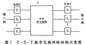
The entire switching network is centered on the S switch. For a switching network with N input multiplexing lines and N output multiplexing lines, 2N sets of T connectors need to be configured, of which N sets are on the input side, which are primary T connectors to complete the user's transmission time slot to The exchange of common time slots inside the switching network; N sets on the output side, called secondary T switches, complete the transfer of the residence on the common time slots inside the switching network to the receiving time slot of another user. Therefore, the number of public time slots provided inside the switching network determines the number of voice channels that can be formed in the switching network. The middle S switch is mainly composed of an N × N cross contact and a control memory bank with N memories, which is used to complete the exchange of user information carried in the switching network from an input side multiplex line to a specified one Output multiplex line.
3 Establishment of mathematical model of TST exchange network
3.1 Description of the problem
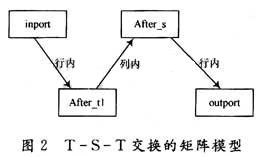
Before establishing the mathematical model of the TST switching network, the mathematical abstraction is first given: the input data stream is represented by an n × n input matrix inport, and each row represents the input link of a TST switching network, that is, each One row represents 1 link HW, and the position of elements in each row represents the order relationship of each data frame in 1 time slot. Since the T exchange is an exchange between different time slots of the same link, it is abstracted as an in-row replacement of the matrix. Therefore, after the input matrix inport undergoes one-level T exchange, an intermediate matrix after_t1 is obtained. This matrix is ​​obtained by inline transformation of each row of data in the import matrix. In the same way, since the S exchange is an exchange between the same time slots of different links, it is similar to performing an intra-column transformation on a matrix in the same column, which is called intra-column replacement. In this way, when after_tl goes through S exchange again, another intermediate matrix after_s is obtained, which is obtained by in-column transformation of the after_tl matrix. Finally, after the second level of T exchange, the outport matrix is ​​generated. Similarly, it is obtained by in-row transformation of the after_s matrix. Therefore, the exchange algorithm can be described as follows: For the initial matrix inport, how to find a transformation method that satisfies the TST three-level exchange, and finally get an output matrix outport. And for any outport required by the user (this matrix is ​​in unicast relationship with inport), the transformation method can be found through the algorithm, that is, two intermediate matrices can be found.
3.2 Establishment of matrix model
The T transform corresponds to the in-row transform of the matrix, and the S transform corresponds to the in-column transform of the matrix, so the above statement can be described as the inport matrix undergoes a series of in-row transforms to obtain the after_t1 matrix, and the after_t1 matrix undergoes a series of columns The internal transformation obtains the after_s matrix, and the after_s matrix undergoes a series of in-row transformations to obtain the export matrix as shown in FIG. 2.
4 Design idea of ​​exchange algorithm
As can be seen from the above discussion, this article has abstracted the specific path selection problem into a purely mathematical problem. Next, this article will find an algorithm from a purely mathematical point of view to solve this exchange problem.
4.1 Mathematical analysis of the problem
Observe the entire transformation process from input matrix inport → intermediate matrix after_t1 → intermediate matrix after_s → output matrix outport. The input matrix has undergone 2 time transformations and only 1 spatial transformation. That is to say, when an element in the input matrix inport needs to undergo column transformation, he has only one chance of transformation. This situation is applicable to any element in the inport. Therefore, the time transformation only plays an adjustment role, so this article will focus on the spatial transformation and try to find the characteristics of the matrix from the spatial transformation S transformation.
It is not difficult to find that the intermediate matrix after_s (n × m) (in general, this article takes m = n, non-blocking switched network) has such characteristics: n elements of each column, and their row numbers include from 1 to n All line numbers. You can see this in the example above. In this way, when the after_s matrix undergoes a spatial transformation and transforms in the reverse direction of the spatial transformation, the n elements will return to the original row in the import matrix, and after an inverse transformation of the temporal transformation can become Inport for the input matrix.
After discovering the characteristics of the intermediate matrix after_s, there is a basic idea. As long as the algorithm here can make the export matrix be transformed into a matrix that satisfies the characteristics of the intermediate matrix after_s after 1 time transform inverse transform, then it will also find a matrix transformation method. Solved this exchange problem. Is there a problem of transforming from inport to outport, can it be converted to a problem that can meet the requirements of the after_s matrix, this after_s matrix is ​​only obtained after a time transformation of the export matrix.
In this way, for any input matrix inpott, any output matrix outport can be obtained after three transformations in the rows, columns, and rows of the matrix, thereby successfully completing TST exchange. In order to facilitate the description of the core algorithm of inport and TST exchange, we may define inport as an order matrix n × n, that is, in order of behavior, from 0 to n × n-1, for example n = 4, inport is defined as:

The outport will be any permutation matrix of inport. Here may also assume that the outport is:

In order to transform from the inport matrix to the outport matrix, two intermediate matrices after_t1 and after_s must be found to complete the switching path connection. Therefore, the goal of this paper is to study an algorithm that generates these two intermediate matrices based on the input matrix and output matrix, so that the processor can fill the register array according to the four matrices, so that TST network exchange can be achieved. For convenience of later description, the three register arrays are defined as: Tregister1 (time division), Sregister (space division), Tregister2 (time division).
Because in the actual TST exchange, the CPU completes the exchange according to the values ​​in the various control registers. According to the characteristics of the exchange, the value of each control register is determined by the input sequence and the output sequence. The value of Tregisterl can be determined by inport and after_t1. Similarly, the value of Sregister is determined by after_t1 and after_s, and the value of Tregister2 is determined by after_s and outport.
4.2 Design of algorithm ideas
Algorithm design requirements:
(1) For any given input matrix and output matrix, 2 intermediate matrices can be obtained;
(2) From the input matrix to the first intermediate matrix, only a series of in-row permutations can be performed;
(3) From the first intermediate matrix to the second intermediate matrix, only a series of intra-column permutations can be performed;
(4) From the second intermediate matrix to the output matrix, only a series of in-row permutations can be performed.
The properties of the after_t1 (AT) and after_s (AS) matrices can be inferred from the properties of in-row transformation and in-column transformation:
Features of AT: ATIj = INij '(can only be replaced on the same row); Features of AS: AS is a substitution matrix of inport; elements in the same row of inport cannot appear on the same column of AS.
This is because it is impossible for inport elements on the same row to appear in the same column of AT, but the conversion from AT to AS is performed within the column.
Now with inport and outport, the goal is to find after_t1 and after_s through these 2 matrices. From the above design requirements and the characteristics of the two intermediate matrices of the model, it can be seen that the permutation from inport to outport and the permutation from outport to inport are symmetrical, so the two intermediate matrices obtained from outport to inpott permutation It is also the solution to the problem. Moreover, inport is more certain than output, so in order to facilitate the description and algorithm implementation, this article uses the inverse method, after_s is inversely derived from outport through a series of in-row transformations, and after_t1 is inferred from after_s through a series of in-row transformations. It is easy to find that from after_s to after_t1 only needs a simple sort to complete, so the key to the algorithm is to derive after_s from the export.
In this way, the key problem to be solved by the switching network scheduling algorithm studied in this paper is equivalently decomposed into: transforming an arbitrary permutation matrix into a permutation matrix of the same row of data in the same column without the input matrix (this is Determined by the characteristics of AS). The algorithm to solve this key problem is called the core algorithm of the switching network scheduling algorithm.
5 Ideas and steps of the key matrix algorithm
5.1 High Conflict Value Row Priority Arrangement Algorithm
Some conventions and definitions:
Rule: There is no data in the same row of the matrix inport on the same column of the matrix after_s.
Then for any given output matrix outport (OP), the task of this algorithm is to put each row element of the outport in the appropriate position of the peer after_s (AS) according to the "rules". For example, assuming that the arrangement of the i-th row starts now, that is to say, the data from the 0th row to the i-lth row has been initially placed (considering the traceback, so "preliminary"), then the elements of each column of the previous i The initial matrix rows can form a one-dimensional matrix, a total of n one-dimensional matrices, defined as a vertical row array v [0], v [1]. …, V [n-1]; and the initial matrix row of all elements of the i-th row of the OP can form a one-dimensional matrix (the initial matrix row of the element is equal to the quotient of the divisor of the element), defined as Line array h, the data structure is shown in Figure 3:
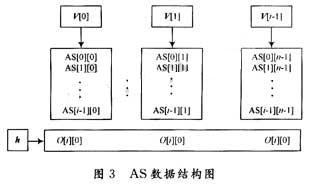
Definition: Vertical conflict value: vRepeat [n], where vRepeat [i] (i = 0, 1, 2, ..., n-1) is equal to the sum of the number of repetitions of the elements in u [i] in h.
Horizontal conflict value: hRepeat [n], where hRepcat [i] (i = 0, 1, ..., n-1) is equal to the sum of the number of repetitions of k [i] in v.
Lifenum: Assume that vRepeat [j] is equal to k, that is to say, there are k elements in O [i] that cannot be placed in the jth column of AS, and the number of elements that can be placed in this column is only nk, defined For the survival number (lifenum), the subscripts of the nk elements are taken out to form a vector, which is defined as the lifespace.
5.2 Implementation of high-conflict value row prioritization algorithm
When the algorithm places the data elements, it starts with the column with the largest vRepeat and then the largest hRepeat with the "rules", and then the smaller columns in the vRepeat with the "rules". In this way, elements with large conflict values ​​are placed preferentially, and the possibility of rearrangement or backtracking is greatly reduced.
5.2.1 Main process
(1) Arrange the first row of data, row = 0;
(2) row = row + 1, if row≥n, stop, otherwise go to the next step;
(3) Calculate the conflict value, call the backtracking algorithm to determine whether to backtrack, if backtracking, call the backtracking algorithm, otherwise go to the next step;
(4) Select the column with the largest vRepeat conflict value, and place the largest element in hRepeat according to the "rules";
(5) Update vRepeat and hRepeat;
(6) Determine whether the data in this line are all installed, if yes, go to (2), otherwise go to (3).
5.2.2 Judge the backtracking algorithm
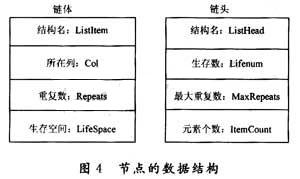
Backtracking condition: The survival number is k, and the number of columns with the same survival space and greater than the survival number k, then backtracking, because a certain survival space is "not enough to allocate". For example, the survival number of the i-th column and the j-th column (i is not equal to j) are both 1 and the survival space is {2}, so that the second element can only be placed in one position, that is, no matter what the arrangement None of them can meet the "rules" and need to go back.
Define the node data structure as shown in Figure 4:
Judging the backtracking algorithm flow:
(1) String all nodes with the same survival number into a linked list, the sequence number of the linked list is equal to the survival number;
(2) Scan the linked list sequentially from the linked list number 0 to the linked list number n, and count the number of nodes with the same survival space. When the number of nodes is greater than the survival number, you need to backtrack, otherwise go to the next step;
(3) Incorporate this chain into the next list;
(4) If all the linked lists do not have the same number of nodes with the same survival space and greater than the number of survival, there is no need to backtrack.
5.2.3 Backtracking algorithm
Defining the experience table: the sequence of positions where each element has "stayed" during the backtracking process.
Backtracking algorithm process:
(1) Determine the traceback element (the principle of maximum conflict value);
(2) Find a "legal location" for the traceback element;
Legal conditions:
Rule: The conflict value is less than the current situation; the location is not in the experience table.
(3) Find "legal positions" for other elements;
6 Proof of algorithm correctness and complexity analysis
From the previous analysis, we can know that the key to solving the entire exchange algorithm is to determine and find the intermediate matrix after_s, that is to say, before solving the problem, it must be determined that the problem has a solution. How to determine that after_s must exist, here we can prove that there must be such a matrix through the principle of drawer in combinatorial mathematics. The proof process is relatively simple, and this article does not make derivation proof here.
From the previous theoretical analysis, we know that there are two important indicators for measuring the exchange algorithm: the number of exchanges and the number of comparisons. In order to count the performance of the exchange algorithm studied in this paper, this paper makes systematic statistics on the exchange times and comparison times of different order matrices:
(1) For each row of data, since the statistical conflict value, the judgment backtracking algorithm and the element placement algorithm are all polynomial complexity, so in the absence of backtracking, this algorithm is polynomial complexity.
(2) In this algorithm, "conflict" plays a very important role, and it avoids many backtracking possibilities. Even if backtracking, the number of positions where "backward" elements are available for backtracking elements and non-backtracking elements is very limited, so the space for backtracking of elements is very small.
The following article gives the statistical results of the average exchange times and comparison times of 50 times when the order of high-conflict row prioritization algorithm changes incrementally without backtracking, as shown in Table 1.
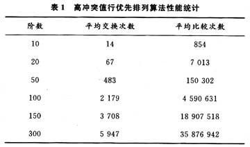
It can be seen from the previous description of the algorithm that the algorithm avoids many possibilities of rearrangement by making each element "find" as much as possible to fit its own position. For a row, the entire arrangement is completely avoided and greatly reduced Backward probability. For most (about 80%) matrices, there is no backtracking. Only a matrix like this can be backtracked (or may not be backtracked), that is, some rows of the AS can be selected from the initial Too few lines. Therefore, the algorithm is an approximate polynomial algorithm, and it is a polynomial algorithm without backtracking. The algorithm can basically complete the path connection of the switching network. He has a great advantage that the number of times of switching in the switching process is minimized, which greatly improves the efficiency of finding the switching path. This algorithm has good characteristics, and can be realized by chip cascading.
Best Ethernet Cable for Gaming,Outdoor Ethernet Cable,Wireless Ethernet Cable,Best Lan Cable
Dong guan Sum Wai Electronic Co,. Ltd. , https://www.sw-cables.com